How to Change the Color of a Bar Graph in Google Sheets
Customizing Your Bar Graph
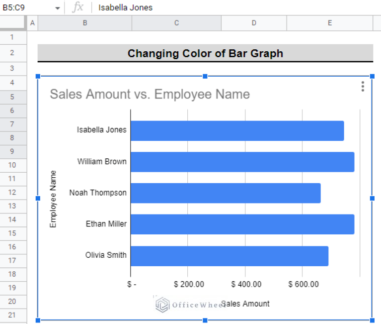
Google Sheets is a powerful tool for creating interactive and dynamic spreadsheets. One of its most useful features is the ability to create visualizations, such as bar graphs, to help illustrate your data. However, the default colors used in these graphs may not always be the most visually appealing or effective. Fortunately, changing the color of a bar graph in Google Sheets is a relatively simple process.
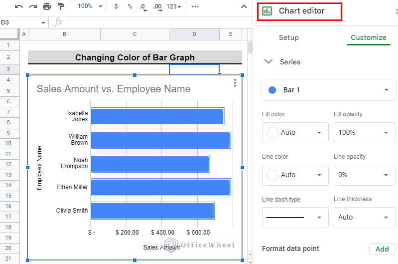
To get started, select the bar graph you want to modify by clicking on it. Then, click on the 'Three vertical dots' icon in the top-right corner of the graph and select 'Advanced edit'. This will open up the 'Chart editor' sidebar, where you can customize various aspects of your graph, including the colors used. In the 'Chart editor', click on the 'Series' tab and then select the series you want to change the color for.
Advanced Color Options
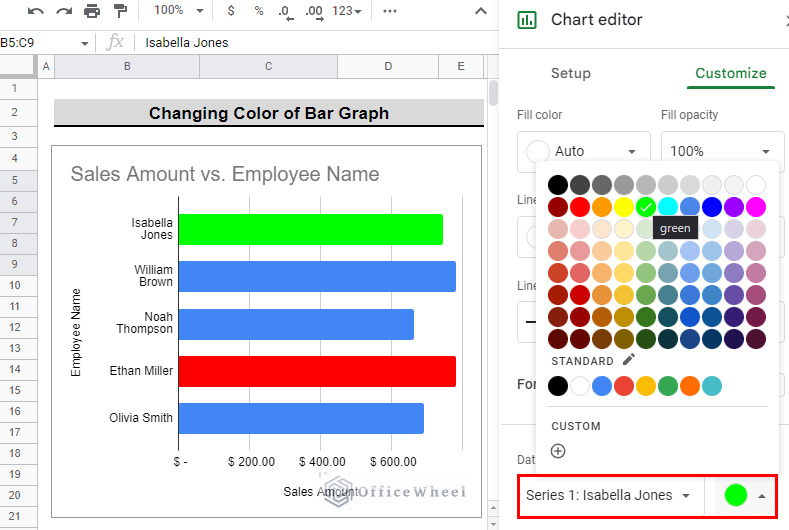
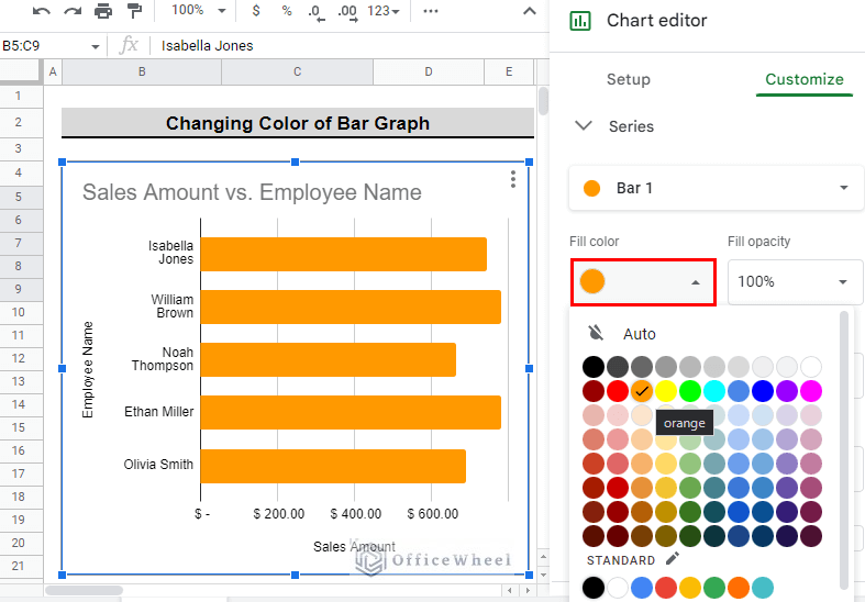
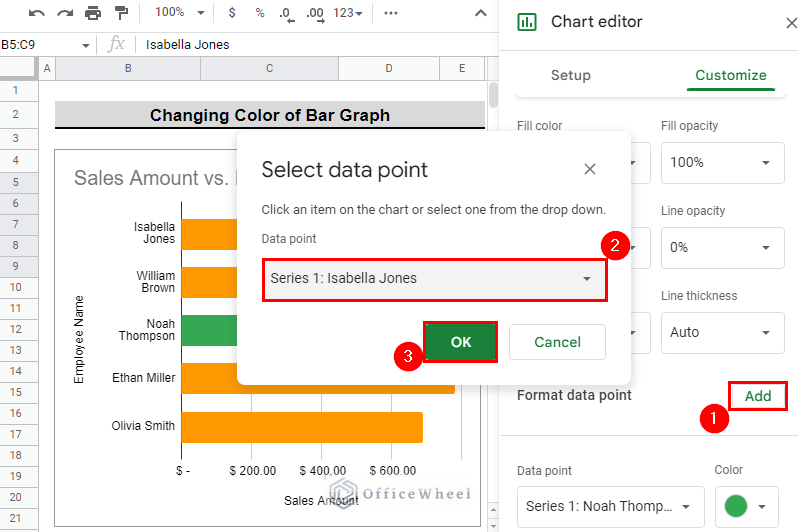
In the 'Series' tab, you can select a predefined color palette or choose a custom color using the 'Color' dropdown menu. If you want to use a custom color, simply click on the 'Custom color' option and enter the hex code or RGB values for the color you want to use. You can also use the 'Default' option to reset the color to its original state. Additionally, you can use the 'Add series' button to add multiple series to your graph, each with its own unique color.
For more advanced color options, you can use the 'Theme' tab in the 'Chart editor' to select from a range of pre-defined themes. These themes can help to give your graph a more cohesive and professional look. You can also use the 'Customize' tab to fine-tune the appearance of your graph, including the colors used for the background, gridlines, and other elements. By using these advanced color options, you can create a bar graph that is not only visually appealing but also effectively communicates your data to your audience.