How To Create A Pie Chart In Google Sheets

Step-by-Step Guide to Creating a Pie Chart

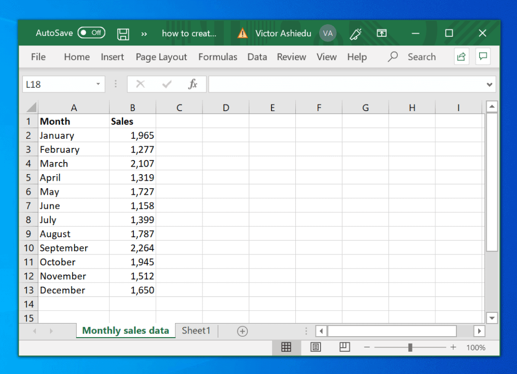
Creating a pie chart in Google Sheets is a great way to visualize your data and make it easier to understand. A pie chart is a circular chart that shows how different categories contribute to a whole. In this article, we will walk you through the steps to create a pie chart in Google Sheets.

To start, select the data range that you want to use for your pie chart. This should include the categories and the corresponding values. Then, go to the 'Insert' menu and select 'Chart'. Google Sheets will automatically create a chart based on your data. However, by default, it will create a column chart or a bar chart. To change it to a pie chart, click on the 'Chart type' button and select 'Pie chart'.

Customizing Your Pie Chart

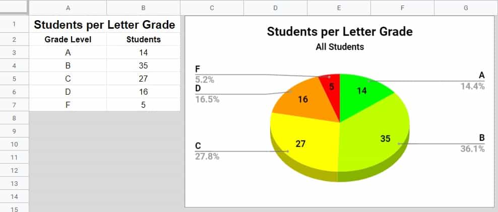
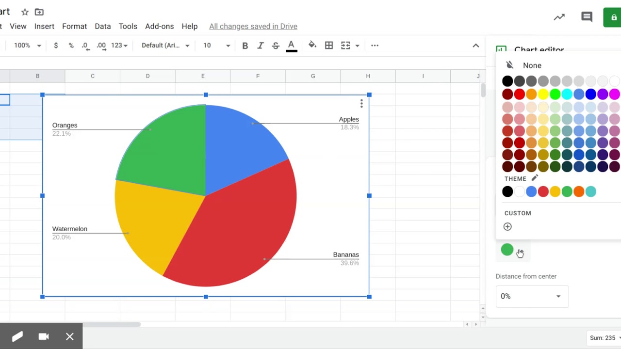
Now that you have created your pie chart, you can customize it to make it look more visually appealing. You can change the colors, add a title, and adjust the size of the chart. To do this, click on the 'Customize' tab in the chart editor. From here, you can change the colors of the slices, add a title to the chart, and adjust the size of the chart. You can also add data labels to the chart to make it easier to read.

In conclusion, creating a pie chart in Google Sheets is a straightforward process that can help you to better visualize your data. By following the steps outlined in this article, you can create a pie chart that effectively communicates your data. Whether you are a business owner, a student, or a researcher, a pie chart can be a powerful tool to help you make informed decisions.