How To Create Chart Formatting In Excel

Understanding Chart Formatting Options

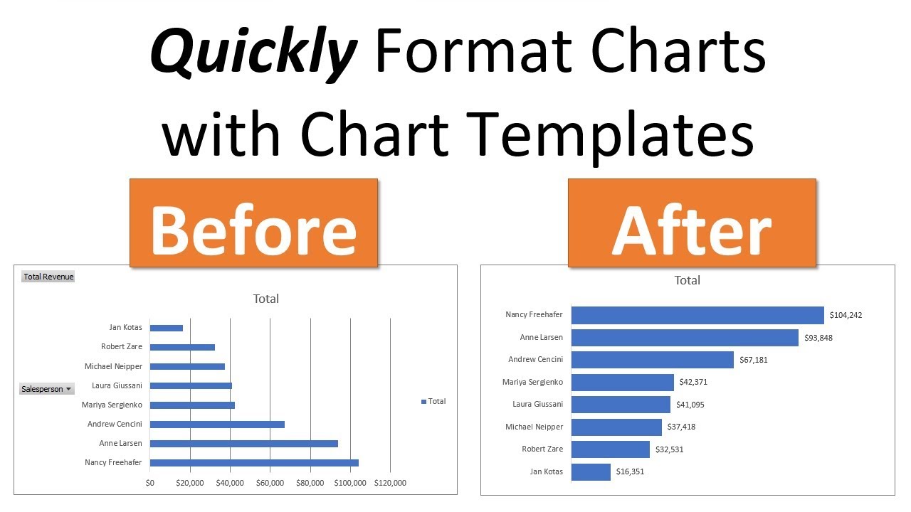
When it comes to presenting data in Excel, charts are an excellent way to visualize trends and patterns. However, a plain chart can be dull and uninteresting. This is where chart formatting comes in - the process of customizing the appearance of your chart to make it more engaging and effective. In this article, we'll show you how to create stunning chart formatting in Excel, making your data stand out and capturing your audience's attention.

To start formatting your chart, you'll need to understand the various options available in Excel. The Chart Tools tab in the ribbon provides a range of formatting options, including colors, fonts, and effects. You can also use the Format tab to customize individual chart elements, such as the title, axes, and data series. By experimenting with different formatting options, you can create a unique and visually appealing chart that showcases your data.

Applying Chart Formatting Techniques

Once you have a good understanding of the formatting options available, you can start applying them to your chart. This is where the real fun begins! You can change the chart type, add colors and textures, and even insert images and shapes. The key is to experiment and find the right balance of formatting elements that enhance your data without overwhelming it. With a little practice, you'll be creating stunning charts that tell a story and convey your message effectively.

By following these simple steps and tips, you can create professional-looking charts that elevate your presentations and reports. Remember to keep your formatting consistent and clean, and don't be afraid to try out new and creative ideas. With Excel's powerful chart formatting tools, the possibilities are endless, and you'll be amazed at how easy it is to create stunning charts that showcase your data in the best possible light.